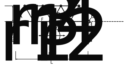
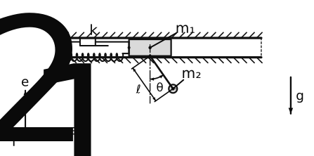
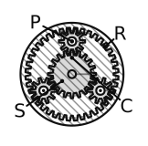
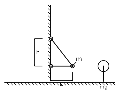
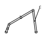
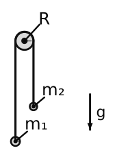
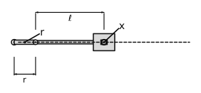
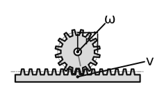
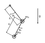
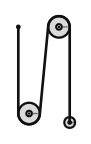
Draw a mechanism once. Simulate it, plot it, publish it.
Ordinate 2D is a free studio where the drawing and the simulation are the same object. Build a pulley system, a linkage or a pendulum on a trolley, and get correct physics in SI units, a textbook-style figure, an animation, live graphs and LaTeX code.
Most tools make you draw the figure in one program and simulate in another, and the two drift apart. Here they cannot.
01
Simulation you can check
Fixed time step, SI units, exact joints and cables, friction, springs, gears and belts. The classic problems are tested against their textbook formulas.
02
Figures like the textbook
Hatched ground, coil springs, dimension arrows, angle arcs, italic labels, LaTeX in any label. Export to SVG, PDF or TikZ.
03
Animations and graphs
Record the motion as video or GIF, plot any quantity live, add stroboscopic snapshots, and export data as CSV or pgfplots.
04
Python, in the browser
Script experiments and parameter sweeps next to the model. It runs on your machine, sandboxed, with nothing to install.
Ordinate 2D NotesStatics · No. 1
Member forces of a Warren truss by the method of joints
Solapsis · worked example
Abstract. A Warren truss carries a load at midspan. We find the support reactions and the force in every member from the equilibrium of the joints, and compare the fifteen forces of a simulation with the hand calculation.
1 Introduction
Truss members are slender bars joined by pins, so each carries only a force along its axis, in tension or compression. The method of joints finds these forces by treating each pin as a particle in equilibrium.
2 Theory
At every joint the forces on the pin sum to zero in both directions:
ΣFx = 0, ΣFy = 0.(1)
For a symmetric truss with a load mg at midspan, each support carries R = mg/2. An end diagonal that makes the angle θ with the horizontal then carries
F = mg2 sin θ (compression).(2)
Figure 1. The truss, with the free-body diagram of the loaded joint P (rod forces Fr and the weight mg).
3 Results
The simulation reproduces the hand calculation for all fifteen members to within 0.002 N. Members at the ends are in compression and the bottom chord is in tension, as expected for a bridge.
References
Hibbeler, R. C. Engineering Mechanics: Statics. Pearson.
Beer, F. P., Johnston, E. R. Vector Mechanics for Engineers: Statics. McGraw-Hill.
Ordinate 2D NotesMechanisms · No. 2
The Peaucellier–Lipkin straight-line linkage
Solapsis · worked example
Abstract. A linkage of seven bars turns circular motion into exact straight-line motion. We show the inversion relation that makes it work and check the traced path in a simulation.
1 Introduction
For almost a hundred years, no one knew whether a linkage could draw an exact straight line. In 1864 Peaucellier found one, and Lipkin found it again in 1871. It needs no guide or slide, only pin joints.
2 Theory
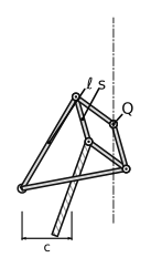
Two long links of length ℓ join the pole O to opposite corners of a rhombus of side s. The two other corners, P and Q, always lie on a line through O, and
OP · OQ = ℓ2 − s2.(1)
The point Q is the inverse of P in a circle about O. A circle through O inverts into a straight line, so if P is guided on such a circle by an extra link, Q moves on a line.
Figure 1. The linkage, exported from Ordinate 2D as SVG.
3 Results
The simulated point Q stays within 1 mm of a straight line over the whole stroke.
References
Kempe, A. B. How to Draw a Straight Line. Macmillan, 1877.
Norton, R. L. Design of Machinery. McGraw-Hill.
Ordinate 2D NotesVibrations · No. 3
Free decay of a damped spring–mass oscillator
Solapsis · worked example
Abstract. A mass on a spring with a viscous damper is released from rest. We give the three regimes of the response and the damped frequency, and compare them with a numerical solution.
1 Introduction
Damping decides whether a vibration rings, returns quickly or creeps back. The ratio of the actual damping to the critical value, ζ, describes all three cases with one number.
2 Theory
The equation of motion for the mass m, spring constant k and damping coefficient c is
mẍ + cẋ + kx = 0.(1)
With ω0 = √(k/m) and ζ = c/(2√(km)), the underdamped motion (ζ < 1) is
x(t) = Ae−ζω0t cos(ωdt + φ), ωd = ω0√(1 − ζ2).(2)
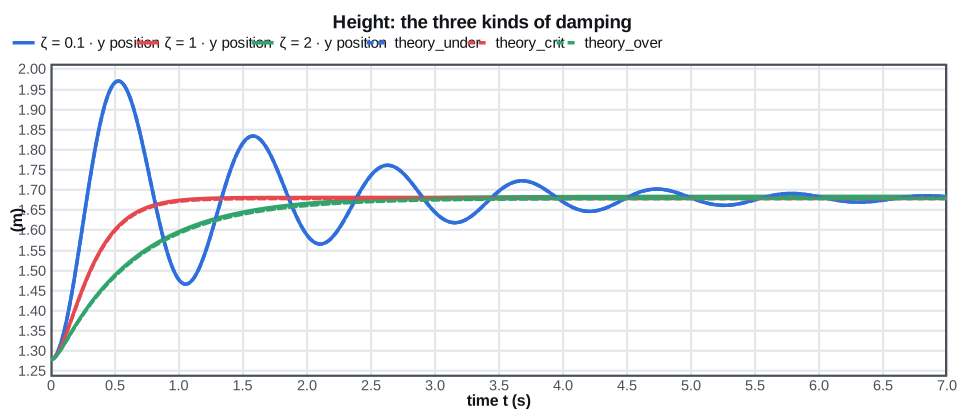
Figure 1. Three dampings, plotted by the studio with their theory curves.
3 Results
Three dampings were simulated: below, at and above ζ = 1. The numerical curves agree with the theory curves. At ζ = 1 the mass returns fastest without overshoot.
References
Thomson, W. T. Theory of Vibration with Applications. Prentice Hall.
Rao, S. S. Mechanical Vibrations. Pearson.
Ordinate 2D NotesStatics · No. 1
Member forces of a Warren truss by the method of joints
Solapsis · worked example
Abstract. A Warren truss carries a load at midspan. We find the support reactions and the force in every member from the equilibrium of the joints, and compare the fifteen forces of a simulation with the hand calculation.
1 Introduction
Truss members are slender bars joined by pins, so each carries only a force along its axis, in tension or compression. The method of joints finds these forces by treating each pin as a particle in equilibrium.
2 Theory
At every joint the forces on the pin sum to zero in both directions:
ΣFx = 0, ΣFy = 0.(1)
For a symmetric truss with a load mg at midspan, each support carries R = mg/2. An end diagonal that makes the angle θ with the horizontal then carries
F = mg2 sin θ (compression).(2)
Figure 1. The truss, with the free-body diagram of the loaded joint P (rod forces Fr and the weight mg).
3 Results
The simulation reproduces the hand calculation for all fifteen members to within 0.002 N. Members at the ends are in compression and the bottom chord is in tension, as expected for a bridge.
References
Hibbeler, R. C. Engineering Mechanics: Statics. Pearson.
Beer, F. P., Johnston, E. R. Vector Mechanics for Engineers: Statics. McGraw-Hill.
Ordinate 2D NotesMechanisms · No. 2
The Peaucellier–Lipkin straight-line linkage
Solapsis · worked example
Abstract. A linkage of seven bars turns circular motion into exact straight-line motion. We show the inversion relation that makes it work and check the traced path in a simulation.
1 Introduction
For almost a hundred years, no one knew whether a linkage could draw an exact straight line. In 1864 Peaucellier found one, and Lipkin found it again in 1871. It needs no guide or slide, only pin joints.
2 Theory
Two long links of length ℓ join the pole O to opposite corners of a rhombus of side s. The two other corners, P and Q, always lie on a line through O, and
OP · OQ = ℓ2 − s2.(1)
The point Q is the inverse of P in a circle about O. A circle through O inverts into a straight line, so if P is guided on such a circle by an extra link, Q moves on a line.
Figure 1. The linkage, exported from Ordinate 2D as SVG.
3 Results
The simulated point Q stays within 1 mm of a straight line over the whole stroke.
References
Kempe, A. B. How to Draw a Straight Line. Macmillan, 1877.
Norton, R. L. Design of Machinery. McGraw-Hill.
Ordinate 2D NotesVibrations · No. 3
Free decay of a damped spring–mass oscillator
Solapsis · worked example
Abstract. A mass on a spring with a viscous damper is released from rest. We give the three regimes of the response and the damped frequency, and compare them with a numerical solution.
1 Introduction
Damping decides whether a vibration rings, returns quickly or creeps back. The ratio of the actual damping to the critical value, ζ, describes all three cases with one number.
2 Theory
The equation of motion for the mass m, spring constant k and damping coefficient c is
mẍ + cẋ + kx = 0.(1)
With ω0 = √(k/m) and ζ = c/(2√(km)), the underdamped motion (ζ < 1) is
x(t) = Ae−ζω0t cos(ωdt + φ), ωd = ω0√(1 − ζ2).(2)
Figure 1. Three dampings, plotted by the studio with their theory curves.
3 Results
Three dampings were simulated: below, at and above ζ = 1. The numerical curves agree with the theory curves. At ζ = 1 the mass returns fastest without overshoot.
References
Thomson, W. T. Theory of Vibration with Applications. Prentice Hall.
Rao, S. S. Mechanical Vibrations. Pearson.
How it works
From idea to figure in three steps
One window: the scene tree on the left, the drawing in the middle, live graphs below and every property on the right.
Ordinate 2D
Draw
Place bodies, springs, ropes, pulleys, gears and joints. Pins snap to surfaces; angles and dimensions are measured for you.
Run
Press Space. Watch the motion, scrub the time bar, read the graphs, and change a number to see what happens.
Export
Take the vector figure into your paper or slides, record the animation, or paste the TikZ code into LaTeX.
Made with Ordinate 2D
Real figures, straight from the studio
Each of these is the studio's own SVG export of a built-in template. Click one to open it, run it and change the numbers.
Over 60 ready-made classic problems are built in, from projectiles and Atwood machines to gear trains and truss bridges, in ten topics:
Motion and projectiles
Forces and friction
Energy, momentum and collisions
Oscillations
Circular motion and rotation
Pulleys, ropes and chains
Statics and structures
Machines and drives
Complex mechanisms
Sandbox and play
For teaching
Built for people who explain mechanics
Exam figures, lecture animations and homework solutions all come from the same model, so they always agree.
Presenter mode for lectures, and PDF export for handouts
Free-body diagrams and member forces in trusses
Parameter sweeps and a data table for lab-style analysis
Nothing to install: students open it in the browser
For research and writing
Publication-quality output
Figures follow the line-art style of classic dynamics books and export as vectors, so they stay sharp in print.
SI units throughout, with a right-handed coordinate frame
LaTeX labels, TikZ and pgfplots export
Scripts and results that you can reproduce
Questions
Frequently asked questions
Is Ordinate 2D free?
Yes. During the beta everything is free: the editor, all templates, the simulation, graphs and every export. A paid plan for publication use is planned; its price will be announced before anything is charged. Compare the plans.
Do I need to install anything?
No. Ordinate 2D runs in a modern desktop browser. During the beta your scenes are stored on your own device, not on our servers; export a scene to keep a copy or to share it. Accounts, with cloud scenes and share links, are coming.
Can I use the figures in lecture notes, exams and homework?
Yes. You may use the studio and its figures free of charge for personal, study and teaching purposes. Terms for publishing figures in books, papers or commercial work will be published before anything is sold; until then, tell us about your use through the updates form.
How accurate is the simulation?
It uses a fixed time step, SI units and exact joints, and the classic problems are tested against their textbook formulas: the fifteen member forces of the Warren truss match the hand calculation to 0.002 N, and the Peaucellier linkage draws its line to within 1 mm. It is a teaching and figure tool, not engineering certification, so check safety-critical results independently.
Which formats can I export?
Figures as SVG, PDF or TikZ code for LaTeX; animations as video or GIF; graphs and data as CSV or pgfplots. Labels can contain LaTeX.
How is it different from PhET, Algodoo or TikZ?
PhET offers polished simulations of one topic each, Algodoo is a playful sandbox, and TikZ draws precise figures from code. Ordinate 2D lets you build any mechanism yourself, simulates it in SI units and draws it in textbook style, from the same model.
Build your first mechanism in a minute
Open a template, press Space, and change a number.